[1]:
import numpy as np
import deeptime.markov.msm as dm
import matplotlib.pyplot as plt
import synd.core
from mr_toolkit.reweighting import splicing
from scipy.special import rel_entr
/home/jd/anaconda3/envs/mr_toolkit/lib/python3.11/site-packages/tqdm/auto.py:22: TqdmWarning: IProgress not found. Please update jupyter and ipywidgets. See https://ipywidgets.readthedocs.io/en/stable/user_install.html
  from .autonotebook import tqdm as notebook_tqdm
NESS Trajectory Splicing
In order to obtain unbiased estimates of a nonequilibrium steady-state distribution, it is not sufficient to compute a transition matrix from equilibrium trajectories and apply recycling boundary conditions to the matrix.
Instead, unbiased estimates require incorporating the boundary conditions into the trajectories, and then computing a transition matrix, which will then naturally contain the appropriate boundary conditions.
Load some pre-discretized sample trajectories
[2]:
trajectories = np.load('sample_data/coarser-sample_trajectories.npy')
Define a set of source and target states
[3]:
state_definitions = np.load('sample_data/coarser-state_definitions.npz')

source_states = state_definitions['source']
target_states = state_definitions['target']
# target_states = np.array([400,401,402])
[4]:
ref_ness = np.load('sample_data/coarser-reference_distributions.npz')['ness']
synd_model = synd.core.load_model('sample_data/coarser-model.synd')
[5]:
lagtime = 10
Standard MSM approach
Obtain a biased estimate, by applying boundary conditions to the transition matrix
[6]:
msm = dm.MaximumLikelihoodMSM().fit_from_discrete_timeseries(trajectories, lagtime)
[7]:
tmatrix = msm.fetch_model().transition_matrix
[8]:
recycling_tmatrix = tmatrix.copy()

recycling_tmatrix[target_states,:] = 0.0
recycling_tmatrix[target_states, source_states] = 1.0

recycling_msm = dm.MarkovStateModel(recycling_tmatrix)
[9]:
biased_ness = recycling_msm.stationary_distribution
Splicing (unbiased) approach
Now, we’ll instead apply the boundary conditions to the trajectories.
[10]:
spliced_trajectories = splicing.iterative_trajectory_splicing(
    trajs=trajectories,
    sink_states = target_states,
    source_states = source_states,
    splice_msm_lag = 1,
    n_clusters = len(tmatrix),
    max_iterations=1000
)
Splicing iteration: 17%|█████████████████████████████████████▉ | 171/1000 [00:06<00:30, 27.62it/s]
(Optionally, backmap the trajectories so you can visualize them in coordinate-space. The coordinate for this model is essentially an RMSD.)
[11]:
spliced_backmapped = synd_model.backmap(spliced_trajectories)
original_backmapped = synd_model.backmap(trajectories)
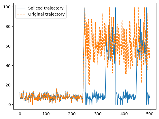
Visualize the spliced trajectories
[12]:
window = 250

target_entry_traj, target_entry_point = np.argwhere(trajectories == target_states[0])[0]

plt.plot(
    spliced_trajectories[
    # spliced_backmapped[
        target_entry_traj,
        target_entry_point-window:target_entry_point+window
    ],
    label='Spliced trajectory'
)

plt.plot(
    trajectories[
    # original_backmapped[
        target_entry_traj,
        target_entry_point-window:target_entry_point+window
    ],
    '--',
    label='Original trajectory'
)

plt.legend()
[12]:
<matplotlib.legend.Legend at 0x7f6bf0dfbf10>
And obtain a Markov estimate from the trajectories.
We toggle on allow_disconnected, because splicing may affect sampling of some states near the target.
[13]:
spliced_model = dm.MaximumLikelihoodMSM(allow_disconnected=True).fit_from_discrete_timeseries(spliced_trajectories, lagtime=lagtime)

spliced_ness = spliced_model.fetch_model().stationary_distribution
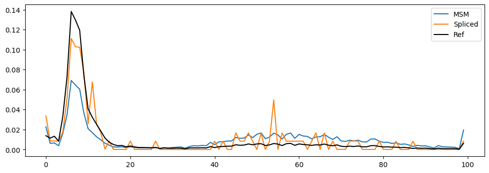
[14]:
plt.plot(biased_ness, label='MSM')
plt.plot(spliced_ness, label='Spliced')
plt.plot(ref_ness, color='k', label='Ref')

plt.gcf().set_size_inches(12,4)
plt.legend()
[14]:
<matplotlib.legend.Legend at 0x7f6bf0e0f7d0>